Rigorous Coupled-Wave Analysis

Overview of RCWA

1. Determine the eigenmodes of each layer by Fourier expansion of the material distribution;
2. Calculate the in-out relation and coupling coefficients of single layer with eigenmodes and the electromagnetic boundary condition;
3. Calculate overall layers by the Redheffer star product;
4. Recover Electromagnetic fields with input light source, global in-out-relation, and coupling coefficients.

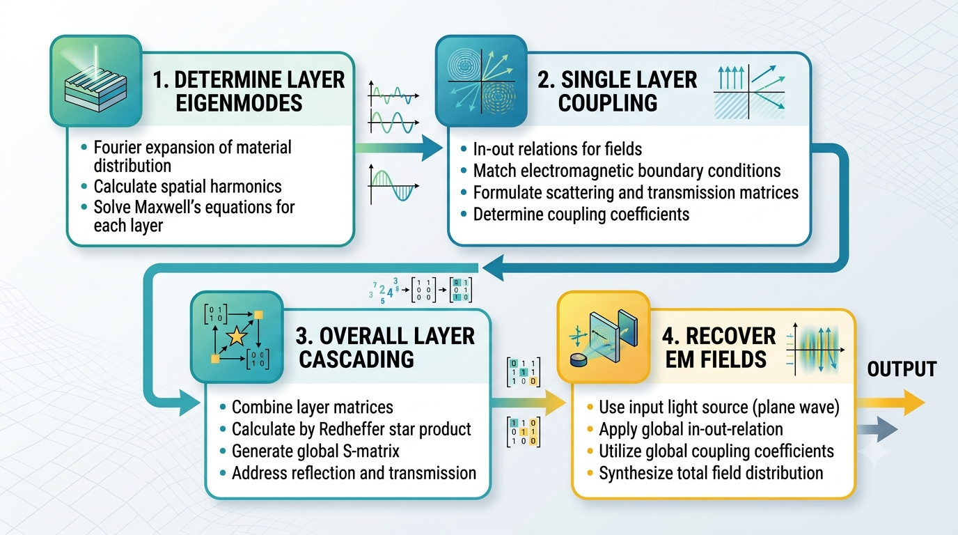
Figure 1. Flowchart of RCWA.

Theory

The relative permittivity and permeability of each layer and the time-harmonic Maxwell’s curl Equations can be expressed as：

$$ \begin{equation} \begin{aligned} & \mu(x,y)=\varepsilon(x+mT_x,y+nT_y), n,m\in{Z}\\ & \varepsilon(x,y)=\varepsilon(x+mT_x,y+nT_y), n,m\in{Z}\\ & \nabla \times \mathbf{E}=j \omega \mu_0 \mu(x, y) \mathbf{H} \\ & \nabla \times \mathbf{H}=-j \omega \varepsilon_0 \varepsilon(x, y) \mathbf{E} \end{aligned} \end{equation} $$

where $T_x, T_y$ is periods of $x,y$ axis, $\omega$ is the angular frequency of the light, $\mu_0,\varepsilon$ is the permeability and permittivity in free space, respectively.

The relative permittivity and permeability of the layer can be expanded as the truncated Fourier series in x- and y-directions as below.

$$ \begin{aligned} & \varepsilon(x, y)=\sum_{m=-2 M}^{2 M} \sum_{n=-2 N}^{2 N} \varepsilon_{m, n} e^{j\left(m G_x x+n G_y y\right)} \\ & \mu(x, y)=\sum_{m=-2 M}^{2 M} \sum_{n=-2 N}^{2 N} \mu_{m, n} e^{j\left(m G_x x+n G_y y\right)} \end{aligned} $$

where $G_x=\frac{2\pi}{T_x},G_y=\frac{2\pi}{T_y}$ are reciprocal lattice vectors in x- and y-directions. M and N are the truncated orders in Fourier harmonics.

$$ U_i(u,v)=U_o(\xi,\eta)\bigotimes h(u,v;\xi,\eta) $$

We transform the Maxwell’s curl Equations into Lorentz-Heaviside units for convenience and to minimize floating-point errors. In this unit, $E$ , $H$ and $\omega$ are different, $E_{SI} \to E_{LH}, \sqrt{\mu_0/\varepsilon_0}H_{SI}\to H_{LH},\sqrt{\mu_0\varepsilon_0}\omega_{SI} \to \omega_{LH}$. Equation (1) can be expressed as,

$$ \begin{aligned} & \nabla \times \mathbf{E}=j \omega \mu(x, y) \mathbf{H} \\ & \nabla \times \mathbf{H}=-j \omega \varepsilon(x, y) \mathbf{E} \end{aligned} $$

The electromagnetic fields in a single layer can be expressed as truncated Fourier series.

$$ \begin{aligned} \mathbf{E} & =e^{j\left(k_{0, x} x+k_{0, y} y+k_z z\right)} \sum_{m=-M}^M \sum_{n=-N}^N \mathbf{E}_{m, n} e^{j\left(m G_x x+n G_y y\right)} \\ \mathbf{H} & =e^{j\left(k_{0, x} x+k_{0, y} y+k_z z\right)} \sum_{m=-M}^M \sum_{n=-N}^N \mathbf{H}_{m, n} e^{j\left(m G_x x+n G_y y\right)} \end{aligned} $$

---

[1] Kim, Changhyun, and Byoungho Lee. “TORCWA: GPU-accelerated Fourier modal method and gradient-based optimization for metasurface design.” Computer Physics Communications 282 (2023): 108552.